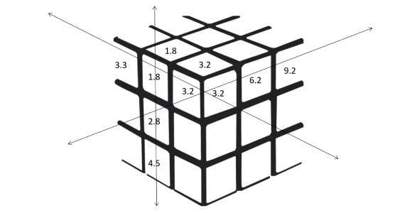
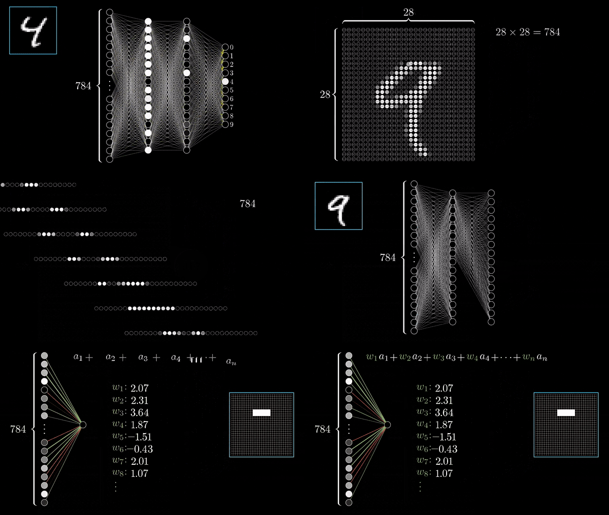
Deep Learning is a subfield of machine learning concerned with algorithms inspired by the structure and function of the brain called artificial neural networks. In this series of articles let us dive deep into PyTorch and learn to train a small neural network to classify images.

If you are new to PyTorch, let me explain it: PyTorch is a Python-based scientific computing package that mainly serves two broad purposes:

• A replacement for NumPy to use the power of GPUs and other accelerators.

• An automatic differentiation library that is useful to implement neural networks.

Why PyTorch?

Well, It is widely accepted that PyTorch is the DeepLearning framework of the Future. PyTorch is designed to provide good flexibility and high speeds for deep neural network implementation. It is open source and is based on the popular Torch library.

PyTorch is different from other deep learning frameworks that it uses dynamic computation graphs, whereas other frameworks like Tensorflow use static computation graphs.

PyTorch is also comparatively easy to learn, easy to debug and has a large community to support.

Let's Build some "BASICS" :

TENSORS:

PyTorch tensors are similar to NumPy arrays with additional features such that they can be used on Graphical Processing Unit or GPU to accelerate computing.

The main difference between a PyTorch Tensor and a numpy array is that a PyTorch Tensor can run on a CPU as well as a GPU. If you want to run the PyTorch Tensor on Graphical Processing Unit you just need to cast the Tensor to a CUDA datatype.

CUDA stands for Compute Unified Device Architecture. CUDA is a parallel computing platform and application programming interface model created by Nvidia. It allows developers to use a CUDA-enabled graphics processing unit.

INITIALIZATION OF A TENSOR:

import torch
import numpy as np

//Initializing directly from data
data = [[1, 2], [3, 4]]
x_data = torch.tensor(data)

TENSOR ATTRIBUTES:

tensor = torch.rand(2,6)

print(f"Shape of tensor: {tensor.shape}") //tensor.shape -> ([2,6])
print(f"Shape of tensor: {tensor.dtype}") //torch.float32
print(f"Shape of tensor: {tensor.device}") //cpu

WE CAN MAKE OUR TENSORS WORK ON GPU:

//We move our tensor to the GPU if available
if torch.cuda.is_available():
  tensor = tensor.to('cuda')
  print(f"Device tensor is stored on: {tensor.device}") //GPU

INTRODUCTION TO AUTOGRAD (TORCH.AUTOGRAD):

torch. autograd is PyTorch’s automatic differentiation engine that powers neural network training.

Neural Networks - NN are a collection of nested functions that are defined by parameters consisting of weights and biases, which in PyTorch are stored in tensors.

Training of NN happens in two steps:

Forward Propagation: In forward propagation, the NN makes its best guess about the correct output. It runs the input data through each of its functions to make this guess.

Backward Propagation: In backpropagation, the NN adjusts its parameters proportionate to the error in its guess. It does this by traversing backward from the output, collecting the derivatives of the error with respect to the parameters of the functions (gradients), and optimizing the parameters using gradient descent.

FORWARD AND BACKWARD PROPAGATION IN PYTORCH:

We load a pre-trained resnet18 model from torchvision. We create a random data tensor to represent a single image with 3 channels, and height & width of 64, and its corresponding label initialized to some random values. Label in pre-trained models has shape (1,1000).

import torch, torchvision
//initializing model
model = torchvision.models.resnet18(pretrained=True)
//initializing data
data = torch.rand(1, 3, 64, 64)
labels = torch.rand(1, 1000)

Now, we run the input data through the model through each of its layers to make a prediction. This is the forward pass.

prediction = model(data)  //forward pass

Then, We use the model’s prediction and the corresponding label to calculate the error (loss). The next step is to backpropagate this error through the network. We implement backpropagation through, .backward() on the error tensor.

Autograd then calculates and stores the gradients for each model parameter in the parameter’s .grad attribute.

loss = (prediction - labels).sum() //sum up all the losses
loss.backward() //backward pass

Now we load the optimizer to modify each epoch's weights and minimize the loss function. Here we use SGD (Stochastic gradient descent) with a learning rate of 0.01 and momentum of 0.9.

optim = torch.optim.SGD(model.parameters(), lr=1e-2, momentum=0.9)

Finally, we call .step() to initiate gradient descent. The optimizer adjusts each parameter by its gradient stored in .grad.

optim.step() //gradient descent

At this point, you have everything you need to train your neural network. Let us explore the Construction of Neural networks and building our model to classify images in PyTorch in the next part.

OUTRO:

In this tutorial, we learned what PyTorch is, and what its advantages are. We also discussed tensors and Autograd in PyTorch. I believe this gave you a basic understanding of PyTorch as a framework. As I have mentioned above, PyTorch is a widely popular and progressive deep learning framework for the future.

related resources:

Thank you for reading 😊

HAPPY LEARNING

-JHA